Using Bayesian analysis to investigate the probability that Nadal wins a point on his own serve against Novak Djokovic at the French Open.

Priors

Since our unknown parameter is \(p\), which is always between 0 and 1, I will use Beta as the prior distribution.

For the non-informative scenario 1, a reasonable prior for \(p\) is \(Uniform(0,1) = Beta(1,1)\) since it gives an equal probability to all values between 0 and 1, which reflects the lack of knowledge.

Given the information in scenario 2, we can find good parameters for the prior that fit the given constraints.

target_mean <- 46/66

alphas <- seq(0.1, 60, length.out = 500)
betas <- (1-46/66)*alphas/(46/66)

param_df <- tibble(alphas, betas)

param_df <- param_df |> mutate(vars = 
                    (alphas*betas)/((alphas + betas)^2*(alphas + betas + 1)))


target_var <- 0.05657^2

param_df <- param_df |> mutate(dist_to_target = abs(vars - target_var))

param_df |> filter(dist_to_target == min(dist_to_target))

# A tibble: 1 × 4
  alphas betas    vars dist_to_target
   <dbl> <dbl>   <dbl>          <dbl>
1   45.4  19.7 0.00320     0.00000374

\(Beta(45.36,19.72)\)

Given the information in scenario 3, we can find good parameters for the prior that fit the given constraints.

Generate possible pairs of alpha and beta values that result an a mean of 0.75

Recall that the mean of a Beta distribution is calculated using: \(\frac{\alpha}{\alpha + \beta}\)

alpha <- seq(0.001, 300, length.out = 1000)
beta <- 0.25*alpha/0.75
possible_params <- tibble(alpha,beta)

Given we are “almost sure” that Nadal wins no less than 70% of his points on serve against Djokovic, we want \(P(p < 0.70)\) to be a small value, and I am going with 0.02

possible_params %>% 
  mutate(probs = pbeta(0.70, alpha, beta)) %>%
  mutate(dist_to_target = abs(probs - 0.02)) %>%
  filter(dist_to_target == min(dist_to_target))

# A tibble: 1 × 4
  alpha  beta  probs dist_to_target
  <dbl> <dbl>  <dbl>          <dbl>
1  252.  83.9 0.0200      0.0000289

\(Beta(251.65,83.88)\)

	Non-Informative Prior	Informative Prior 1	Informative Prior 2
\(\alpha\)	1	45.35511	251.6518
\(\beta\)	1	19.71961	83.88394
Mean	0.5	0.69697	0.75

Data

From class, we know we can update the prior distribution based on our data. If \(y_{obs}\) is the number of points won:

\(g(p|y_{obs}) = Beta(y_{obs} + \alpha, n - y_{obs} + \beta)\)

\(y_{obs} = 56\)

\(n = 84\)

The mean is equal to \(\frac{\alpha}{\alpha + \beta}\):

Carry out the math…

	Non-Informative Posterior	Informative Posterior 1	Informative Posterior 2
\(\alpha\)	57	101.3551	95.03965
\(\beta\)	29	47.71961	41.01322
Mean	0.6627907	0.6798947	0.7333149

	Non-Informative Posterior	Informative Posterior 1	Informative Posterior 2
Prior Mean	0.5	0.69697	0.75
Posterior Mean	0.6627907	0.6798947	0.6985494

All of the posterior means are between their prior mean and our value from the data (\(\frac{56}{84} = 0.667\)), which makes sense.

90% Credible Intervals

# non informative
c(qbeta(0.05, 57, 29),qbeta(0.95, 57, 29))

[1] 0.5772453 0.7440061

# informative 1
c(qbeta(0.05, 101.3551, 47.71961), qbeta(0.95, 101.3551, 47.71961))

[1] 0.6158797 0.7411561

# informative 2
c(qbeta(0.05, 307.6518, 111.8839), qbeta(0.95, 307.6518, 111.8839))

[1] 0.6972162 0.7681476

Report

In this project our end goal is to try and find the “true” distribution for the probability that Nadal wins a point on his own serve against Novak Djokovic at the French Open. The probability distribution for winning points given he takes \(n\) serves can be modeled using a Binomial distribution, with parameters \(n\) and \(p\) where \(p\) is the probability of Nadal winning the point for a single serve.

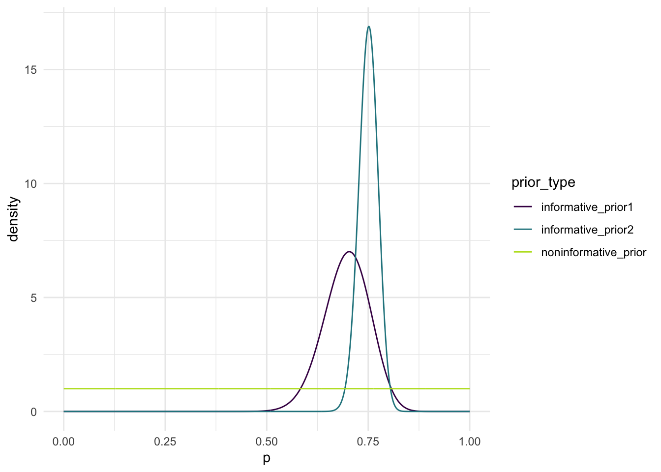
The parameter \(p\) is our unknown that we want to find the distribution for. Before using our data, we need a prior that we can update with said data. For this project we have priors for 3 different scenarios. But for all 3 scenarios, we can use a Beta distribution to model as we know the value of \(p\) can only be between 0 and 1. We can look at each resulting distribution and evaluate which we think best models Nadal’s performance, and these final distributions will be affected by the priors we choose.

For the non-informative prior, I used a \(Beta(1,1)\), which is the same as a \(Uniform(0,1)\). This gives an equal probability for all values of \(p\) since we assume we “know nothing” about the distribution before collecting any data.

For the first informative prior we are given previous data where Nadal won 46/66 points on his serves against Djokovic, so we can treat this as the mean. There is also a standard error of 0.05657 on this estimate. We can use this information to find a prior that fits these constraints. We know that the mean of a Beta distribution is equal to \(\frac{\alpha}{\alpha + \beta}\). If we set this equal to 46/66 we can solve for \(\alpha\) in terms of \(\beta\). We can then run through values of \(\alpha\) and calculate the corresponding \(\beta\) that keeps the mean at 46/66. Then select the \(\alpha\) \(\beta\) pair with the variance closest to \(0.05657^2\). This gave a prior of \(Beta(45.36, 19.72)\).

For the second informative prior we are given a value of 0.75 to work with, and we can treat this as the mean. From the second piece of information we know that \(P(p < 0.70)\) is a small value, so I used 0.02. Then similar to how we did the first informative prior, calculate \(P(p < 0.70)\) for combinations of \(\alpha\) and \(\beta\) and select the combination that has \(P(p < 0.70)\) closest to 0.02. This gave a prior of \(Beta(251.65, 83.88)\).

Comparing the Posteriors

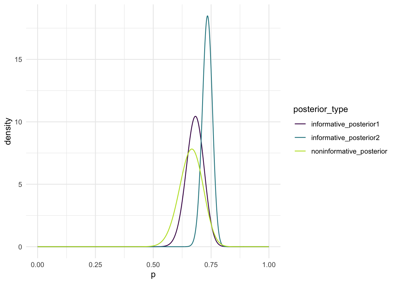
The three posterior distributions are all different because we started with different priors (different \(\alpha\) and \(\beta\) values). In class we figured out how to update our distribution using our data:

\(g(p|y_{obs}) = Beta(y_{obs} + \alpha, n - y_{obs} + \beta)\)

So we can see that although each prior is updated in the same way, the initial \(\alpha\) and \(\beta\) values will have a strong influence on the resulting posterior.

Choosing a Posterior

Based on the three posteriors, I would choose the first informative one. Although the second informative prior has the lowest variance by a fair margin (see below), it is only based on the claims of the commentator. So yes the distribution has a small variance, but this smaller range of values that the 90% credible interval covers may be inaccurate. The first informative one’s prior was based on real (?) data from previous matches between Nadal and Djokovic, and for this reason I would pick it over both of the other options. It reflects known past performance of Nadal versus Djokovic, and based on the real data we have, the interval seems more reasonable. This first informative scenario gives us data to use where p = 0.667, and this value is not even in the credible interval for the second informative scenario.

Posterior Variance

\(Variance = \frac{\alpha\beta}{(\alpha + \beta)^2(\alpha + \beta + 1)}\)

variance <- function(alpha, beta) {
  var = (alpha*beta)/((alpha + beta)^2*(alpha + beta + 1))
  return (var)
}
# non-informative
variance(noninformative_alpha, noninformative_beta)

[1] 0.002568956

# informative 1
variance(informative_alpha1, informative_beta1)

[1] 0.001450197

# informative 2
variance(informative_alpha2, informative_beta2)

[1] 0.0004650358

The variance for the second informative posterior is lower than the variance for the other two because its prior started with a much lower variance. From the first graph you can see that the curve for the second prior is much taller and narrower, indicating a low variance. This makes sense because we knew the peak had to be “centered” over 0.75 and have only 2% of the density below 0.70, which is not far from 0.75. So although the distribution was adjusted by the observed data, 0.667 is not too far from 0.75, so the distribution stayed narrow. Since the distribution started with a relatively high confidence in Nadal’s performance, it remained high.